As of version 1.3, dbt supports the usage of python models. This significantly extends the capabilities of what you can achieve with dbt. This blog will discuss the potential of using dbt’s new Python functionality to enable machine learning in your data projects. 

After this blog, you should 

• Be convinced of the benefits of using Python models in your dbt project; 
• Have the knowledge to implement Python models yourself.

Additionally, we will provide a code example from one of our own projects. More specifically, we recently implemented Facebook's Prophet algorithm, an advanced SARIMA model, right into our dbt Cloud project to forecast client demand for caretakers in different municipalities based on historical trends.

Why Python in dbt?

Initially, this may seem strange. Transforming, structuring, and cleaning data is typically achieved with SQL. Even though it is possible with Python, SQL is known to be much more efficient in quickly handling large amounts of data. However, when it comes to machine learning, Python’s rich open-source library of pre-build packages allows you to easily implement advanced machine learning techniques right into your projects. While SQL beats Python in terms of raw data querying performance, Python beautifully complements this strength by enabling the implementation of advanced machine learning techniques on that same data. As of recently, both dbt and Snowflake have enabled the writing and executing of Python code directly into their environments, enabling engineers to effectively use A.I. right in their Snowflake data warehouse. This effectively allows developers to build end-to-end mini machine learning pipelines right in their dbt Cloud projects.

Python models

In dbt, a python model functions exactly as any other SQL model would, meaning it serves the same exact place in a DAG and suffers from the same limitations (more on that later). Python models can also reference one or more upstream SQL models and can be referenced by downstream models using dbt’s built-in ref function. Similar to the SQL models, Python models are created by adding the .py suffix and have to reside in dbt’s models folder. While a typical .sql model would look something like this:

SELECT *

FROM {{ ref('ml_pre_clientdemand') }}

where ml_pre_clientdemand is a regular upstream SQL model, a python model has a slightly more complex base structure:

def model(dbt, session):

    dbt.config(materialized = "table", packages = ["pandas"])

    referenced_table = dbt.ref("ml_pre_clientdemand")

    df = referenced_table.to_pandas()

    #Python magic here!

    return df


A few things to note here:

1. The model parameters dbt and session are required and not to be changed;
2. A dbt config block is used to configure the model as well as denote any third-party packages you might want to use;
3. The ORGADMIN of the target Snowflake account must enable the use of third-party Python packages –> Using Third-Party packages in Snowflake
4. The model has to return a single data frame, which will be materialized in your (Snowflake) data warehouse. This is identical to a SQL model as they too only “return” a single table;
5. Once a SQL model is referenced (referenced_table in the code snippet above) and converted into a data frame, all Python is fair game.
6. In a dbt lineage graph, a Python model is indistinguishable from any other regular SQL model:

Machine learning models

Now that we have a basic understanding of how Python models work in dbt, it is time to take it up a notch. Python’s open-source library of packages makes more advanced matters such as machine learning and A.I. easily accessible to anyone wanting to try their hands on it. Popular packages like Facebook’s Prophet, Amazon’s deepAR, Scikit-learn, Scipy, Pandas, and even Pytorch and Tensorflow make it easier than ever for data engineers to implement machine learning in their data projects to solve all kinds of problems. Typical use cases may include:

1. Data clustering to group similar clients,
2. Classification to predict cancer in patients based on a collection of biomarkers,
3. Anomaly detection to detect fraud or machine defects,
4. Time series forecasting to predict future client demand based on historic data,
5. …

Since both dbt and Snowflake now allow the full usage of Python, we can set up an end-to-end machine learning pipeline right in our own dbt Cloud/Snowflake environment. The next section will go into more detail about how we used Python models to set up an end-to-end machine learning-based forecasting system to predict future client demand for caretakers in each municipality in Flanders, Belgium.

Reference case: Time series forecasting to predict client demand

A client active in-home care wants to predict future client demand for each municipality in Flanders to steer and match employee availability to avoid having employees without clients and clients without a caretaker. By predicting client demand in each municipality, they would be able to move employees who have too few clients from one municipality to another so that client demand meets employee availability. To aid in their migration to the Cloud, the following basic structure was set up:

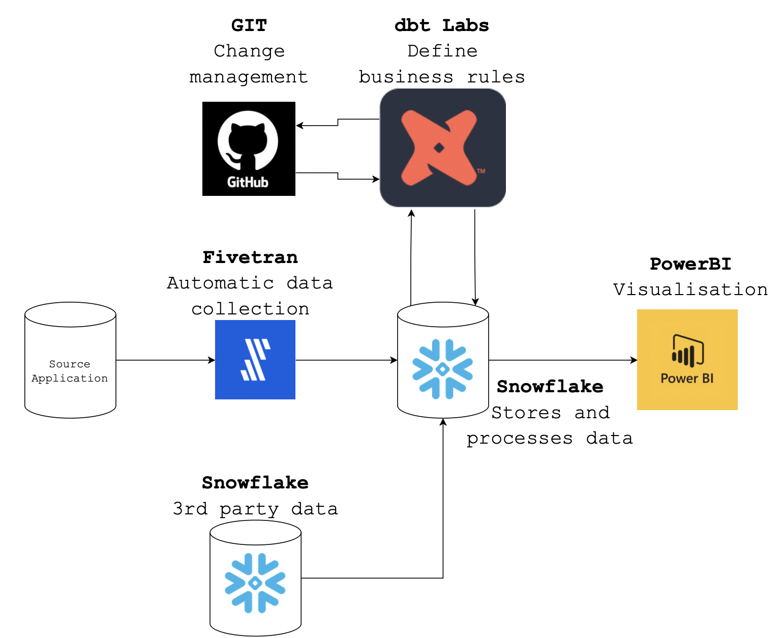
Using dbt Cloud, source data containing raw client and employee information is ingested into Snowflake. Next, the raw data is modeled using a collection of regular SQL models into a familiar star schema or party-event model. From the modeled data, flat tables are derived in a preprocessing step and staged to be used in a forecasting algorithm. Here, historic client demand per municipality is chronologically ordered and collected in one big table. Once the data has the right shape and format, a Python model containing the Prophet forecasting algorithm is trained on each municipality and predicts client demand for the next few months. The figure below shows the full DAG build in dbt Cloud to achieve this goal. 

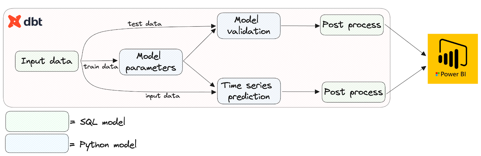
There are three Python models present in the DAG, all with very different purposes:

1. model_paramaters refers to the Python model that houses the main training loop. It returns a dataframe with a single cell, saving the trained model parameters to be loaded in at a later stage;
2. model_validation, as the name suggests, calculates relevant performance metrics by comparing the trained model’s predictions with the actuals in the test data set;
3. time_series_predictions returns the actual model predictions based on the input data.

A code example of the model_parameters model is shown below:

import pandas as pd

from prophet import Prophet

import numpy as np

from datetime import datetime

def train_predict_prophet(df, periods):

    df_prophet_input = df[['ds', 'y']]

    model = Prophet()

    model.fit(df_prophet_input)

    future_df = model.make_future_dataframe(

        periods=periods, 

        include_history=False)

    forecast = model.predict(future_df)

    return forecast

def min_max_scaling(column):

    if column.min() == column.max():

        return [1] * len(column)

    return (column - column.min())/(column.max() -  column.min())

def model(dbt, session):

    dbt.config(materialized = "table", packages = ["pandas", "numpy", "prophet"])

    my_sql_model_df = dbt.ref("ml_pre_clientdemand")

    df_main = my_sql_model_df.to_pandas() #CONVERT TO DATAFRAME DATATYPE

    df_main['DATE'] = pd.to_datetime(df_main['DATE'], format='%Y-%m-%d') #CONVERT TO CORRECT DATEFORMAT

    df_main = df_main.sort_values(by=['MUNICIPALITY', 'DATUM'])

    df_main = df_main.rename(columns={"DATUM": "ds", "KLANT_VRAAG": "y"}) #RENAME DATUM AND VAL COLUMNS TO DS AND Y FOR PROPHET

    unique_regional_cities = df_main.MUNICIPALITY.unique()

    unieke_regionale_steden= df_main.REGIONALE_STAD.unique()

    union = pd.DataFrame()

    for regionale_stad in unique_regional_cities:

        for gemeente in unique_municipalities:

            df_municipality = df_main.loc[(df_main['REGIONAL_CITY'] == regionale_stad) & (df_main['MUNICIPALITY'] == municipality)]

            if municipality.shape[0] == 0:

                continue

            #SCALAR FOR DENORMALIZATION AND EXTRACT CURRENT REGION

            unique_regions = df_municipality.REGIO.unique()

            current_region = unique_regions[0]

            #NORMALIZE DATASET TO CONSIST OF VALUES 0-1

            df_municipality_history_deep = df_municipality.loc[(df_municipality['ds'] < datetime.strptime("2020-01-01", '%Y-%m-%d'))]

            df_municipality_history = df_municipality.loc[(df_municipality['ds'] >= datetime.strptime("2020-01-01", '%Y-%m-%d')) &       (df_gemeente['ds'] < datetime.strptime("2022-01-01", '%Y-%m-%d'))]

            df_municipality_current = df_municipality.loc[(df_municipality['ds'] >= datetime.strptime("2022-01-01", '%Y-%m-%d'))]

            scalar = df_municipality_current['y'].max() - df_municipality_current['y'].min() 

            term = df_municipality_current['y'].min() #descaling occurs by: scalar * val + ter

            if scalar < 0.001: # aka scalar is zero

                scalar = df_municipality_current['y'].max()

                term = 0

            df_municipality_history_deep['y'] = min_max_scaling(df_municipality_history_deep['y'])

            df_municipality_history['y'] = min_max_scaling(df_municipality_history['y'])

            df_municipality_current['y'] = min_max_scaling(df_municipality_current['y'])

            df_municipality = pd.concat([df_municipality_history_deep, df_municipality_history, df_municipality_current])

            #TRAIN PROPHET AND RETURN FORECAST

            forecast = train_predict_prophet(df_municipality, 160)

            #ADD CHARACTERIZING COLUMNS TO FORECAST

            forecast['REGION'] = [current_region] * len(forecast)

            forecast['REGIONAL_CITY'] = [regional_city] * len(forecast)

            forecast['MUNICIPALTY'] = [municipality] * len(forecast)

            forecast['ISFORECAST'] = [1] * len(forecast)

            forecast['SCALAR'] = [scalar] * len(forecast)

            forecast['TERM'] = [term] * len(forecast)

            #UNION HISTORIC DATA AND FORECAST

            union = pd.concat([union, forecast])

    union = union.reset_index(drop=True)

    union['ds'] = union['ds'].dt.date

    union = union.rename(columns={"ds": "DS", "y": "Y", "yhat":"YHAT", "yhat_lower":"YHAT_LOWER", "yhat_upper":"YHAT_UPPER"})

    return union

A few things to note here:

• As can be seen above, while def model(dbt, session) function is required, there is no limit on the number of self-defined functions you can use;
• While as much preprocessing as possible should be done in the upstream SQL models for performance purposes, some light preprocessing and postprocessing can be done if the situation demands it. Examples are casting date formats to pandas date format, renaming columns as Prophet demands the value column to be called y and the date column to be called ds, or collecting the forecast results in a manner easily processable in downstream models;
• The packages defined in the dbt model’s config block and those imported at the top of the file the old-fashioned way have the exact same functionality. However, by importing packages at the top, they allow you to set abbreviations for certain names (like renaming pandas to pd, numpy to np…).

Once the output of the forecast and the validation metrics has been collected, post processing steps are performed in a few final SQL models before the resulting tables are sent to a visualization tool. The image below shows the actual predictions for future client demand in a normalized form.

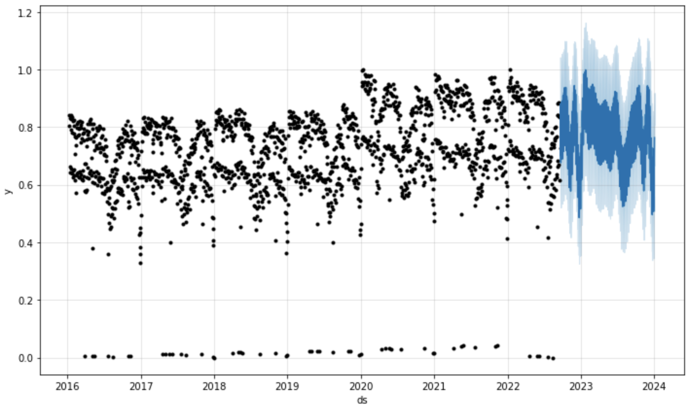
Performance metrics also showed accurate predictions for up to a year after the last observation, implying Prophet correctly captures historic trends to predict future client demand. Although Prophet is still a relatively simple forecasting technique, it opens the door to implementing much more advanced techniques should more complex problems demand it. Amazon’s deepAR or other recurrent and LSTM neural networks have proven to be more accurate and more capable of learning complex patterns. However, training neural networks takes significantly longer and requires a lot more data than we had available.

Drawbacks

Although very feasible, building Python models is tough as dbt is not a fully flushed out Python IDE and provides very little development functionality. Development is therefore recommended locally, using Snowpark to easily access data stored in Snowflake.

Additionally, Python models tend to be slower in execution than regular SQL models. This is mainly due to the fact that dbt wraps your Python code in a procedure construct, followed up by calling that procedure after which the procedure is dropped again. This process is suboptimal causing the general performance of Python models to take a hit. This might be another reason to prefer the direct usage of Snowparks functionality over the usage of Python models.

Final remarks

The introduction of Python models brought a bunch of new functionality to dbt. Advanced analytics not suitable to be carried out with SQL are now easily handled by the addition of dedicated Python models in your DAG. Smaller scale machine learning pipelines can be set up end-to-end right in your dbt Cloud project.